🤳 예전 포스팅에서 '특성공학(feature engineering)'이 무엇인지에 대해 간략하게 개념 학습을 하였다.
FE - Feature Engineering
1. Concepts * In real world, data is really messy - we need to clean the data * FE = a process of extracting useful features from raw data using math, statistics and domain knowledge - 즉, 도메..
sh-avid-learner.tistory.com
🏃♂️ 우리가 실생활의 data를 가지고 모델링하는 machine learning의 세계에서 무수히 많은 feature를 만날텐데, 이 모든 feature를 modeling에 대입하면 model이 터진다..? 기존 우리가 원하는 방식의 model의 성능이 안나올 확률이 높다. 최대한 중요한 feature만 남겨두거나, 기존에 주어진 feature들 일부를 domain knowledge에 의해 재조합해 중요한 feature를 만드는 feature를 이용한 여러 작업을 함으로써 우리는 modeling의 성능을 높일 수 있다고 본다.
👓 이번 포스팅을 통해 우리는 feature selection - 즉 '중요한 특성만 뽑아내는 여러가지 방법' 중 그 첫번째, selectKBest()를 사용하는 것에 대해 알아보려 한다!
▷ selectKBest docu ◁
class sklearn.feature_selection.SelectKBest(score_func=<function f_classif>, *, k=10)
🌂 sklearn에서 제공하는 feature_selection module에서는 다양한 형태의 method를 제공해준다. 그 중 selectKBest()는 univariate feature selection의 일부분으로 모든 feature들 각각 한 개씩 target에 영향을 준다고 가정(각 feature들이 target과의 연관성에 독립적으로 평가됨)할 때(그래서 univariate이다. multivariate이면 scoring할 때 두 개 이상의 변수가 동시에 target에 영향을 준다고 가정하고 시작한다), 이 때의 영향 정도를, 원하는 scoring method로 점수를 매겨서 가장 점수가 높게 나온 feature들 k개만 (default는 10개) 선택하는 함수이다.
'Univariate feature selection works by selecting the best features based on univariate statistical tests. It can be seen as a preprocessing step to an estimator. Scikit-learn exposes feature selection routines as objects that implement the transform method'
selectKBest removes all but the K highest scoring features
👁 여기서 target 속성에 따라, 즉 regression인지 classification인지에 따라 적용하는 score_func가 다르다
→ regression) f_regression / mutual_info_regression
→ classification) chi2 / f_classif / mutual_info_classif
'The methods based on F-test estimate the degree of linear dependency between two random variables'
= f-분포를 가정하고 두 변수간의 선형적 의존성 정도를 산출하는 (앞에 f_가 붙으면) scoring method이다.
<<다양한 score_func>>

Q. categorical type data가 있으면 selectKBest를 수행할 수 없을까?
A. 어렵다
→ 각종 docu와 많은 article들 Q&A를 찾아봤지만, categorical data type을 따로 one-hot 또는 ordinal 등등 encoded되는 과정이 거치질 않는다면 selectKBest 수행이 어려움.
→ 따라서 selectKBest 과정 이전에 먼저 encoding하는 전처리 과정을 거치고 난 뒤 수행 추천!
→ 에러는 아래와 같이 뜸
'ValueError: Unable to convert array of bytes/strings into decimal numbers with dtype='numeric'
FutureWarning: Arrays of bytes/strings is being converted to decimal numbers if dtype='numeric'. This behavior is deprecated in 0.24 and will be removed in 1.1 (renaming of 0.26). Please convert your data to numeric values explicitly instead.
X = check_array('
(+) numeric data라면 discrete & continuous 모두 selectKBest 수행 가능
-- 직접 예시와 함께! --
① 원하는 scoring method와 kBest를 import
from sklearn.feature_selection import f_regression, SelectKBest
② selector 객체 정의 (즉 어떤 method로 몇 개를 뽑을 건지 뽑으려는 '일종의 안내서(객체)' 만들기)
selector = SelectKBest(score_func=f_regression, k=10)
③ 해당 안내서를 가지고 train, test (val도 있다면 모두) 또는 전체 data에 적용
(처음에는 fit_transform → transform - fit는 한 번만 해서 select하는 방법을 적용시키면 이후 transform만 수행하면 됨!)
## 학습데이터에 fit_transform
X_train_selected = selector.fit_transform(X_train, y_train)

## 테스트 데이터는 transform
X_test_selected = selector.transform(X_test)
④ 감소된 feature들 결과 data shape() 확인
(이젠 X_train_selected로 modeling을 수행하면 된다.)
X_train_selected.shape, X_test_selected.shape++ selector 유용한 method 살펴보기 ++
get_support()
** 중요! get_support()는 어떤 특성들이 선택되었는 지, 선택되면 True, 아니면 False를 반환해준다. 따라서 해당 method를 통해 어떤 특성들이 선택되었는 지 알 수 있다.
selected_mask = selector.get_support()

all_names = X_train.columns

## 선택된 특성들
selected_names = all_names[selected_mask]

## 선택되지 않은 특성들
unselected_names = all_names[~selected_mask]
그 외 fit()와 transform()을 활용해서 X와 y를 집어넣어 알맞는 feature들을 선택한다
++ 추가) 가장 score가 높게 나온 attribute 출력하기
<< numpy.argmax()>> 사용!
selector.feature_names_in_[selector.scores_.argmax()]
<<top n개의 score나온 attribute 출력하려면 .argsort()[-n:]>>
selector.feature_names_in_[selector.scores_.argsort()[-n:]]
#n개의 top score features
<<뒤에서 n개의 가장 적은 score들이 나온 attribute 출력하려면 .argsort()[:n]>>
selector.feature_names_in_[selector.scores_.argsort()[:n]]
#score값 적은 n개의 feature names
++ seaborn - jointplot으로 두 변수간의 correlation 시각화 ++
∽ jointplot docu ∽
https://seaborn.pydata.org/generated/seaborn.jointplot.html
seaborn.jointplot(*, x=None, y=None, data=None, kind='scatter', color=None, height=6, ratio=5, space=0.2, dropna=False, xlim=None, ylim=None, marginal_ticks=False, joint_kws=None, marginal_kws=None, hue=None, palette=None, hue_order=None, hue_norm=None, **kwargs)
🤖 "Draw a plot of two variables with bivariate and univariate graphs"
≫ 주로 수치형 연속형 두 변수간의 관계를 육안으로 바로 파악하고 싶을 때 사용한다!
"kind{ “scatter” | “kde” | “hist” | “hex” | “reg” | “resid” }"
≫ 여러 종류의 graph로 두 변수간의 관계를 jointplot에 나타낼 수 있으며 주로 numerical bivariates' correlation을 나타내기 위해 회귀선이 scatterplot에 포함된 형태로 많이 사용한다 (kind = 'reg')
예제) <k selection에 따른 성능 실험>
Q. 주어진 car price data와 만들어진 MLR 모델에서 car price를 결정지을 유용한 변수들만 f_regression에 의해 몇 개를 뽑는게 좋을 지 selectKBest에 의해서 구하는 feature selection을 진행한다. 이후 결정한 evaluation metric에 의해 feature selection 이전과 이후 얼마나 MLR 모델 성능이 좋아졌는지 수치를 통해 확인하자. the number of features에 따른 error 수치의 변화를 그래프로 시각화하고 과적합이 일어나지 않는 최적의 모델 성능을 보이는 feature의 개수 및 해당 선택된 feature의 종류를 구해보자.
(+추가 작업 - jointplot 시각화를 근거로 selectKBest에 의해 selected된 feature의 정당성을 보이자)
A.
1> import & dataset 준비
import pandas as pd
import matplotlib
import seaborn as sns
import numpy as np
import matplotlib.pyplot as plt

path = 'https://cf-courses-data.s3.us.cloud-object-storage.appdomain.cloud/IBMDeveloperSkillsNetwork-DA0101EN-SkillsNetwork/labs/Data%20files/module_5_auto.csv'
df = pd.read_csv(path)
df.to_csv('module_5_auto.csv')
df=df._get_numeric_data()
2> train / test set 나누기 & target과 그 이외의 data로 나누기
train = df.sample(frac=0.75,random_state=1)
test = df.drop(train.index)

train.dropna(inplace=True)
test.dropna(inplace=True)

target = 'price' #y는 car price data

## X_train, y_train, X_test, y_test 데이터로 분리
X_train = train.drop(columns=target)
y_train = train[target]
X_test = test.drop(columns=target)
y_test = test[target]
3> evaluation metrics는 r2 score & MAE / 그리고 1개부터 전체 column까지 차례로 selectKBest 돌려 각각의 training set & test set의 지표 결과 시각화하기
from sklearn.feature_selection import f_regression, SelectKBest
from sklearn.linear_model import LinearRegression
from sklearn.metrics import mean_absolute_error, r2_score
training=[]
testing=[]
feature_names = []
x = range(1, len(X_train.columns)+1)
for num in range(1, len(X_train.columns)+ 1):
selector = SelectKBest(score_func=f_regression, k=num)
X_train_selected = selector.fit_transform(X_train, y_train)
X_test_selected = selector.transform(X_test)
selected_mask = selector.get_support()
selected_names = all_names[selected_mask]
feature_names.append(selected_names)
model = LinearRegression()
model.fit(X_train_selected, y_train)
y_train_pred = model.predict(X_train_selected)
train_mae = mean_absolute_error(y_train, y_train_pred)
training.append(train_mae)
y_test_pred = model.predict(X_test_selected)
test_mae = mean_absolute_error(y_test,y_test_pred)
testing.append(test_mae)
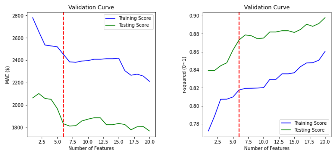
plt.plot(x, training, label='Training Score', color='b')
plt.plot(x, testing, label='Testing Score', color='g')
plt.axvline(6.0, 0, 1, color='red', linestyle='--', linewidth=2)
plt.ylabel("MAE ($)")
plt.xlabel("Number of Features")
plt.title('Validation Curve')
plt.legend()
plt.show()
print('------selected feature names------')
for a in feature_names[5].values[0:6]:
print(a)
4> 결과 해석
🧸 validation curve 시각화 결과(MAE)를 보았을 때 feature 개수가 늘어날수록 이에 과적합되어 error가 결국은 쭉 감소하는 것을 볼 수 있다. 하지만 overfitting의 문제 & 모델 training time의 감소 효율성을 위해 features 수가 적게 선택되는 게 좋기 때문에 error가 큰 폭으로 감소하는 시점인, features 수가 6개일 때가 최적의 feature selection (selectKBest()로만 보았을 때)라고 판단할 수 있다. 여기서 test set error가 제일 적은 20이 제일 좋은 것이 아닌가 라고 생각할 수 있지만 여기서의 test set은 validation 개념이며, 추후 그 어떤 새로운 개념의 test set이 와도 위와 같이 무조건 error가 적게 나온다고 보장이 어렵고 또 실제 세계에서는 이렇게 예측 가능성 설명력이 높은 경우가 드물기 때문에 최소 feature 수의 적정값 내에서 select하는 것이 최적이라고 생각된다. r-squared 시각화 결과를 보았을 때도 test set line에서 결정계수값이 갑작스럽게 증가한 feature가 6개일 때의 지점이 제일 최적이라 생각하며 이후 r-sqaured 결정계수가 소폭 증가하긴 하나 그 정도가 약하므로 그 영향을 배제해도 충분하다고 판단된다. 🧸
(++ r-squared & MAE 관련 오류 지표 상세한 내용은 아래 포스팅 참조 ++ - 추후 adjusted-R metric도 다룰 예정 - ✌️ )
All About Evaluation Metrics(1/2) → MSE, MAE, RMSE, R^2
** ML 모델의 성능을 최종적으로 평가할 때 다양한 evaluation metrics를 사용할 수 있다고 했음! ** (supervised learning - regression problem에서 많이 쓰이는 평가지표들) - 과정 (5) - 😙 그러면 차근차..
sh-avid-learner.tistory.com
→ code 결과 최적의 6개 feature는 'width & curb-weight & engine-size & horsepower & highway-mpg' & 'city-L/100km'
5> jointplot으로 선택된 특성과 target과의 회귀선 시각화 (scatterplot 포함)
<위 선택된 특성 중 horsepower, 그리고 선택 안된 특성 중 compression-ratio를 각각 jointplot으로 시각화한 결과>
#code source by Bhavesh Bhatt
from scipy import stats
from scipy.stats.stats import pearsonr

def plot_join_plot(df, feature, target):
    j = sns.jointplot(feature, target, data=df, kind='reg')
    #j.annotate(stats.pearsonr) 사라짐..
    return plt.show()

train_df = pd.concat([X_train, y_train], axis=1)

plot_join_plot(train_df, 'compression-ratio','price')
plot_join_plot(train_df, 'horsepower','price')

👉 horsepower는 선택된 특성에 맞게 price에 따른 양의 상관관계를 대체적으로 보여주는데 반해, compression-ratio는 회귀선의 기울기가 거의 0으로 price의 변화에 따른 compression-ratio 변화가 거의 없다고 봐도 무방하기 때문에 selectKBest가 선택된 특성에서 제외했다고 볼 수 있다.
- 더 다양한 feature selection 기법 추후 포스팅 예정 🦾 -
* 출처) https://www.kaggle.com/jepsds/feature-selection-using-selectkbest
* kBest 출처) https://www.youtube.com/watch?v=UW9U0bYJ-Ys
* jointplot - 출처) https://www.geeksforgeeks.org/python-seaborn-jointplot-method/
'Machine Learning > Fundamentals' 카테고리의 다른 글
| PCA(concepts) (0) | 2022.05.30 |
|---|---|
| Feature Selection vs. Feature Extraction (0) | 2022.05.18 |
| Ordinal Encoding (0) | 2022.04.20 |
| train vs. validation vs. test set (0) | 2022.04.18 |
| Gradient Descent (concepts) (+momentum) (0) | 2022.04.18 |

댓글