👏 저번 시간에 PCA의 개념 및 주축을 찾기까지의 자세한 과정을 여러 방면으로 분석해보고 알아보았다.
PCA(concepts)
* dimensionality reduction 기법 중 대표적인 방법인 PCA에 대해서 알아보자! concepts> ① 고차원의 data를 낮은 차원으로 차원 축소하는 기법 (dimensionality reduction) ② 기준이 되는 정보는 data의 분산! (분산
sh-avid-learner.tistory.com
👏 이제는 직접 code로 실행해 scree plot으로 시각화해보고 주어진 unsupervised data를 알맞게 clustering해 실제 data가 PC 축에 맞게 잘 분리가 되는지 체크해보는 과정까지 해 보려 한다!
👏 PCA에 대해서 배웠던 개념을 아래 자세히 6가지의 step으로 나눌 수 있다.
① standardization
(np.mean과 np.std로 직접 연산이 가능 / 또는 sklearn의 StandardScaler() 사용)
② constructing a covariance matrix
(np.cov 사용 / 또는 sklearn의 PCA가 알아서 internally하게 연산해줌)
③ performing eigendecomposition of covariance matrix (decompose the matrix into its eigenvectors & eigenvalues)
(np.linalg.eig 사용 / 또는 위에서 언급한 sklearn의 PCA 함수가 알아서 연산)
④ selection of most important eigenvectors & eigenvalues
(직접 eigenvalue를 나열해 PC를 고르거나 / sklearn의 PCA parameter로 정해놓은 수만큼 PC를 알아서 골라준다)
⑤ constructing a projection matrix (using selected eigenvectors) - feature matrix라고 했음!
⑥ transformation of training/test dataset
Q. diesel을 원료로 사용한 차와 사용하지 않은 차에 대한 정보가 담겨 있는 데이터프레임이 있다. PCA를 사용하기에 적절한 feature columns만 골라 feature reduction을 진행해 단 두 개의 주축 PC1과 PC2만 남겨보자. 그리고, target으로 세웠던 diesel 사용여부를 단 두 개의 새로운 feature(PC1, PC2)로 clustering이 쉽게 가능한지 pca plot과 scree plot 시각화를 통해 clustering problem의 해결 여부 정당성을 보여라.
A.
1> dataset 준비 (null column 제거)
#1) load the dataset
path = 'https://cf-courses-data.s3.us.cloud-object-storage.appdomain.cloud/IBMDeveloperSkillsNetwork-DA0101EN-SkillsNetwork/labs/Data%20files/module_5_auto.csv'
car = pd.read_csv(path)
car.to_csv('module_5_auto.csv')
car=car._get_numeric_data()

#1) + check if there is null data in the dataset
nulls_checked = car.isnull().sum()
nulls_col = nulls_checked[nulls_checked != 0].index[0] #deleting 'stroke' col

car = car.loc[:, car.columns!=nulls_col]
car = car.iloc[:, 3:19]
2> feature와 target 분리하고 feature standardization
(여기서 target은 diesel 사용 여부를 택했으며, 실제 PCA는 target 분리 없이 data 그 자체를 줄이는 데 목적이 있지만, 우리는 PCA의 효과를 증명하기 위해, 단 2차원 만으로도 data가 잘 분리가 되었는 지 확인해보고자 target을 따로 분리하고 후에 시각화할 예정!)
#2) standardization
from sklearn.preprocessing import StandardScaler
target = 'diesel'
# Separating out the features
x = car.loc[:, car.columns != target].values #15 dimensions

# Separating out the target
y = car.loc[:,[target]].values

# Standardizing the features
x = StandardScaler().fit_transform(x)

print(x)
- 표준화 이후의 dataframe number -

3> PCA 진행 (n_components는 2로 설정!)
▶sklearn.decomposition.PCA docu()◀
https://scikit-learn.org/stable/modules/generated/sklearn.decomposition.PCA.html
class sklearn.decomposition.PCA(n_components=None, *, copy=True, whiten=False, svd_solver='auto', tol=0.0, iterated_power='auto', n_oversamples=10, power_iteration_normalizer='auto', random_state=None)
#3) perform PCA
from sklearn.decomposition import PCA
pca = PCA(n_components=2) #dimensionality 15 to 2
principalComponents = pca.fit_transform(x) #perform PCA
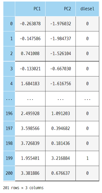
principalDf = pd.DataFrame(data = principalComponents, columns = ['PC1', 'PC2'])
finalDf = pd.concat([principalDf, car[[target]]], axis = 1)
finalDf
4> pca plot & scree plot 시각화 (두 target의 구분을 위해 색상 다르게 입힘)
#4) visualize 2D projection - pca plot
fig = plt.figure(figsize = (8,8))
ax = fig.add_subplot(1,1,1)
ax.set_xlabel('PC1', fontsize = 15)
ax.set_ylabel('PC2', fontsize = 15)
ax.set_title('PCA w/ two components', fontsize = 20)

targets = [0, 1]
colors = ['r', 'b']
for target, color in zip(targets,colors):
    indicesToKeep = finalDf['diesel'] == target
    ax.scatter(finalDf.loc[indicesToKeep, 'PC1']
               , finalDf.loc[indicesToKeep, 'PC2']
               , c = color
               , s = 50)
ax.legend(['no diesel', 'yes diesel'])
ax.grid()
def scree_plot(pca):
    num_components = len(pca.explained_variance_ratio_)
    ind = np.arange(num_components)
    vals = pca.explained_variance_ratio_

    ax = plt.subplot()
    cumvals = np.cumsum(vals)
    ax.bar(ind, vals, color = ['#00da75', '#f1c40f',  '#ff6f15', '#3498db']) # Bar plot
    ax.plot(ind, cumvals, color = '#c0392b') # Line plot

    for i in range(num_components):
        ax.annotate(r"%s" % ((str(vals[i]*100)[:3])), (ind[i], vals[i]), va = "bottom", ha = "center", fontsize = 13)

    ax.set_xlabel("PC")
    ax.set_ylabel("Variance")
    plt.title('Scree plot')

scree_plot(pca)

5> 시각화 결과 분석
👉 총 15개의 feature가 존재하는 car data를 variance를 가장 잘 설명하는 단 두 개의 축, PC1과 PC2만으로 뽑아내어 시각화했다. 그 결과, PC1만으로는 diesel 사용 유무를 정확히 판별할 수 없었지만, PC2 주축이 더해진다면 diesel 유무가 극명히 clustering될 수 있음을 pca plot을 통해 유추할 수 있다.
👉 scree plot으로 시각화한 결과 역시 PC1만으로는 전체 variance의 약 54%만 설명될 수 있음을 알 수 있다. 여기에 PC2 17%가 더해진 합계 약 70%의 설명력으로 diesel 사용 유무가 clustering이 가능함을 알 수 있다.
👉 dataset 자체 양으로만 봤을 때는 diesel이 있을 경우의 data가 압도적으로 비중이 적게 차지해, 애초에 data target 불균형 문제가 생겼다. 좀 더 균일한 target 분포의 data와 충분한 갯수의 data가 존재했다면 더 좋은 clustering 결과가 나오지 않았을 까 예측해 본다.
🕵️ 추후
→ 실제로 PCA를 통해 data reduction(extraction) 효과를 pca plot과 scree plot을 통해 증명해 보았다! 추후에는 실제 ML 모델링에 적용할 때 PCA 이전과 이후 data를 model에 집어넣었을 경우에 따른 elasped time과 model accuracy의 차이를 증명해보고자 한다 🙌
* 출처1) https://vitalflux.com/feature-extraction-pca-python-example/
* 출처2) https://towardsdatascience.com/pca-using-python-scikit-learn-e653f8989e60
'Machine Learning > Fundamentals' 카테고리의 다른 글
| All About Evaluation Metrics (2/2) → MAPE, MPE (0) | 2022.06.11 |
|---|---|
| Unsupervised Learning (0) | 2022.06.03 |
| PCA(concepts) (0) | 2022.05.30 |
| Feature Selection vs. Feature Extraction (0) | 2022.05.18 |
| feature selection (1) - selectKBest (+jointplot) (0) | 2022.04.20 |

댓글