'Decision Trees (DTs) are a non-parametric supervised learning method used for classification and regression. The goal is to create a model that predicts the value of a target variable by learning simple decision rules inferred from the data features. A tree can be seen as a piecewise constant approximation.'
▩ 앞서 소개했던 model list ▩
👓 SLR 단순선형회귀모델
👓 MLR 다중선형회귀모델
👓 RR 릿지회귀모델
👓 LR 로지스틱회귀모델
🤠 이젠 regression과 classification 동시에 쓰일 수 있는 기법 '결정트리(Decision Tree; DT)' 모델에 대해서 알아보려 한다
* structure & explanation w/ pros & cons
- DT 구조 -
→ input와 output(target)이 모두 존재하는 supervised learning 기법 중 하나
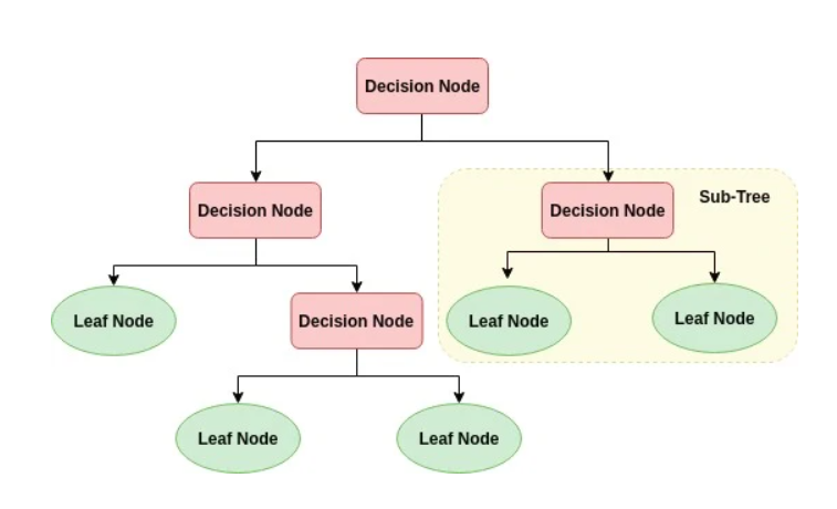
→ 주어진 input(data)에 대해 여러 특성들 중 골라서 한 특성에 대한 분류, 또는 수치를 기준으로 계속 나누어가는, 일종의 스무고개와 같이 분류해 나가 정답 class, 또는 정답 target을 결정하는 모델
→ 데이터를 위 그림처럼 여러 기준들에 대해 분할해가는 알고리즘
→ 결정트리의 각 data의 집단을 node라고 부르며, 뿌리(root) 노드 & 말단(terminal, external, leaf) 노드 & 중간(internal) 노드로 나뉨.
《DT의 장단점》 from scikit-learn
장점🙂>
▷ Simple to understand and to interpret. Trees can be visualised. (시각화할 수 있어서 쉽게 이해 가능함 - 직관적임!)
▷ Requires little data preparation. Other techniques often require data normalisation, dummy variables need to be created and blank values to be removed. Note however that this module does not support missing values. (tree model의 장점은 normalization, scaling 등등의 따로 feature 변환 과정이 필요없다는 점. 그저 각 분기마다 주어진 한 feature에 대해 data를 분리하는 모델이므로, 타 feature와 비교할 일이 없기 때문에 굳이 번거롭게 scaling을 통해서 타 feature들과 맞출 필요가 없다. 그리고 결측치에도 큰 영향을 안 받음)
▷ The cost of using the tree (i.e., predicting data) is logarithmic in the number of data points used to train the tree.
▷ Able to handle both numerical and categorical data. However scikit-learn implementation does not support categorical variables for now. Other techniques are usually specialised in analysing datasets that have only one type of variable. See algorithms for more information.
▷ Able to handle multi-output problems.
▷ Uses a white box model. If a given situation is observable in a model, the explanation for the condition is easily explained by boolean logic. By contrast, in a black box model (e.g., in an artificial neural network), results may be more difficult to interpret. (white-box model이어서 모델을 쉽게 이해할 수 있다)
▷ Possible to validate a model using statistical tests. That makes it possible to account for the reliability of the model.
▷ Performs well even if its assumptions are somewhat violated by the true model from which the data were generated.
단점😶>
▷ Decision-tree learners can create over-complex trees that do not generalise the data well. This is called overfitting. Mechanisms such as pruning, setting the minimum number of samples required at a leaf node or setting the maximum depth of the tree are necessary to avoid this problem. (따로 hyperparameter tuning 설정을 안해주면 data 자체에 너무 과적합된 tree가 산출됨. generalization 성능을 높이기 위해서는 따로 여러 설정들을 해줘야 함)
▷ Decision trees can be unstable because small variations in the data might result in a completely different tree being generated. This problem is mitigated by using decision trees within an ensemble. (불안정한 모델. data가 조금의 변동만 있어도 트리 1개만 놓고봤을 때 전혀 다른 형태의 tree가 나옴. 따라서 이를 해결하기 위해선 여러 tree를 모은 RandomForest(Baggin)나 GradientBoosting 앙상블 모델을 활용해야 한다 - 곧 포스팅)
▷ Predictions of decision trees are neither smooth nor continuous, but piecewise constant approximations as seen in the above figure. Therefore, they are not good at extrapolation. (piecewise approximation 형식으로, 즉 이분법적으로 기준대로 자르는 형식으로 알고리즘이 진행되기 때문에 연속적인 결과가 tree에서 산출되지 않음. 따라서 기존 data 범위가 아닌 새로운 범위에 해당되는 data가 들어온다면(extrapolate) 당연히 예측하기에 너무 힘들다. - 따라서 tree model은 interpolate 기법으로만 사용한다는 암묵적인(?) 룰이 있다..)
▷ The problem of learning an optimal decision tree is known to be NP-complete under several aspects of optimality and even for simple concepts. Consequently, practical decision-tree learning algorithms are based on heuristic algorithms such as the greedy algorithm where locally optimal decisions are made at each node. Such algorithms cannot guarantee to return the globally optimal decision tree. (매 분기마다 locally optimum 지점 택해서 진행되는 tree 모델이므로 globally optimum 지점 못 찾을 확률 있음) This can be mitigated by training multiple trees in an ensemble learner, where the features and samples are randomly sampled with replacement.
▷ There are concepts that are hard to learn because decision trees do not express them easily, such as XOR, parity or multiplexer problems.
▷ Decision tree learners create biased trees if some classes dominate. It is therefore recommended to balance the dataset prior to fitting with the decision tree. (class 분류문제에서 한 쪽 class로만 치우친 dataset이 있다면 편향된, 부정확한 tree가 만들어지므로 tree에 집어넣기 전 애초에 class들을 균형잡게 맞추어야 할 필요가 있음)
- 다시 정리하면 - (장,단점 정리)
| Pros | Cons |
| 시각화 - 직관적! | hyperparameter tuning을 안해주면 overfitting 문제점 가능성 높음 |
| normalization, scaling 등 feature 변환이 따로 필요 x | data가 조금만 변해도 model이 unstable |
| numeric & categorical data 모두 적용 가능 | extrapolation 예측에 효율적 x |
| 다중 output 문제 해결 가능 | locally optimum을 택해서 진행 - globally optimum 찾기 어려움 |
| white-box model | imbalanced dataset - 부정확한 tree가 만들어짐 |
| statistical test를 이용해 model 입증 가능 |
≪비선형, 비단조, 특성상호작용을 가지고 있는 data에 용이≫
▷ 선형이 아닌 비선형인 경우 여러 기준에 의해 DT를 이용해 쉽게 분리될 수 있음.
▷ 단조함수는 도중 오르락내리락이 없는, 전체적으로 단조로운 함수 (비단조는 그 반대) - 따라서 비단조인 경우 여러 기준을 정해 오르락내리락 기점을 DT를 이용해 여러 개로 쉽게 나눌 수 있음
▷ 특성상호작용) 앞서 알아본 선형모델을 통해 애초에 가정으로 다중공선성을 배제했지만, DT를 통해 feature간에 상호작용이 있더라도 여러 기준으로 쉽게 쉽게 분리를 할 수 있음.
* cost function (for classification)
! regression은 cost function으로 MSE, 포아송 deviance, MAE를 사용
! 그리고 target variable이 1또는 0과 같은 binary 형태이면 chi method를 비용함수로 사용
(↑추후 사용 예제 포스팅)
아래는 분류를 위해 사용하는 cost function 종류
☝️ tree 알고리즘의 핵심은 '주어진 data(node)를 어떻게 분할하는가?'
= '결정트리의 비용함수를 정의하고 이를 최소화 하도록 분할하는 것'
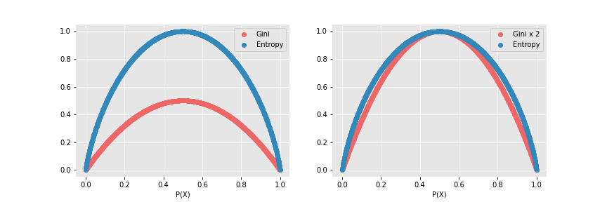
- (좌) 지니 불순도(Gini Impurity (Gini Index)) / (우) 엔트로피(Entropy) -

☆ pi = 주어진 data(분기되는 시점에서의 data)에서의 i 비율 ☆
* 불순도의 개념> '여러 class가 있을 때 다양한 class가 비슷한 비율로 모여 있다면 불순도가 크다고 말할 수 있다. 그만큼 pure하지 않고 다양하게 모여있기 때문. 하지만 한 class가 압도적인 비율을 차지하는 group이라면 상대적으로 더 pure하다고 할 수 있으며, 불순도는 작게 나온다. 한 class만 있는 group은 당연히 불순도가 0이 나옴!
👆 예시 👆
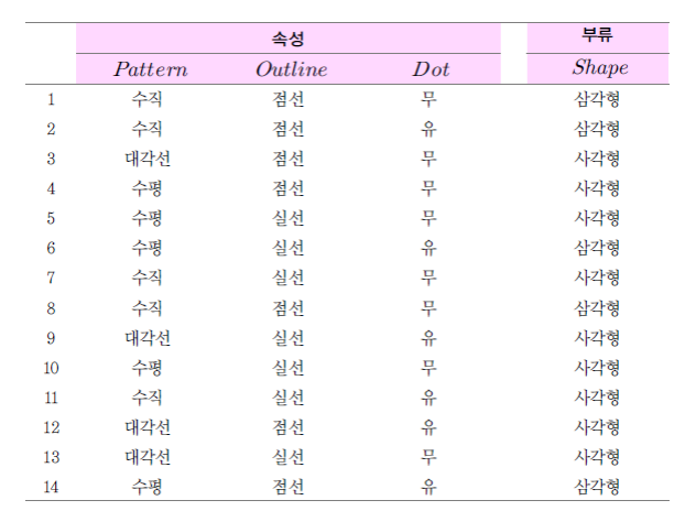
Q. 삼각형과 사각형으로 최종적으로 부류를 나누는 decision tree classifier를 만들고 싶다. 이 때 첫 분류 criteria로 pattern, outline, dot 중 중 어떤 criteria를 고를 지 Gini impurity & entropy 기준으로 각각 골라보자. 그리고 결정된 criteria 종류가 똑같은 지도 확인해보자!
(1) Gini Impurity>
1>> criteria가 Pattern일 경우
① '수직'인 leaf node Gini Impurity = 1 - (3/5)^2 - (2/5)^2 = 0.48
② '수평'인 leaf node Gini Impurity = 1 - (2/5)^2 - (3/5)^2 = 0.48
③ '대각선'인 leaf node Gini Impurity = 1 - (0/4)^2 - (4/4)^2 = 0
* 여기서 Pattern이 criteria일 경우의 total Gini Impurity는 각 leaf node(위)의 weighted average of impurity이다
(각 leaf node의 data 수가 다르기 때문에 이를 고려해야 함)
✍️ total Gini Impurity = weighted average of each leaf nodes' impurity = (5/14)*0.48 + (5/14)*0.48 + (4/14)*0 = 약 0.3429
2>> criteria가 Oultine일 경우
(1>>과 똑같은 방식으로 진행)
① '점선'인 leaf node Gini Impurity = 1 - (4/7)^2 - (3/7)^2 = 0.4898
② '실선'인 leaf node Gini Impurity = 1 - (1/7)^2 - (6/7)^2 = 0.2449
✍️ total Gini Impurity = weighted average of each leaf nodes' impurity = (7/14)*0.4898 + (7/14)*0.2449 = 약 0.3674
3>> criteria가 Dot일 경우
(역시 똑같이 진행)
① '유'인 leaf node Gini Impurity = 1 - (1/2)^2 - (1/2)^2 = 0.5
② '무'인 leaf node Gini Impurity = 1 - (1/4)^2 - (3/4)^2 = 0.375
✍️ total Gini Impurity = weighted average of each leaf nodes' impurity = (6/14)*0.5 + (8/14)*0.375 = 약 0.4286
☀️ 최종적으로 total Gini Impurity가 가장 낮은 criteria를 고른다! <<정답은 Pattern>> ☀️
(2) Entropy> (IG로 분기)
* 엔트로피로도 똑같이 여러 criteria에 맞게 나눠보고 위 entropy 식에 맞게 각 leaf node의 entropy를 계산해보자
1>> criteria가 Pattern일 경우
① '수직'인 leaf node Entropy = -(3/5)log2(3/5) - (2/5)log2(2/5) = 0.971
② '수평'인 leaf node Gini Impurity = -(2/5)log2(2/5) - (3/5)log2(3/5) = 0.971
③ '대각선'인 leaf node Gini Impurity = -(0/4)log2(0/4) - (4/4)log2(4/4) = 0
✍️ total Entropy = weighted average of each leaf nodes' Entropy = (5/14)*0.971+ (5/14)*0.971+ (4/14)*0 = 약 0.694
2>> criteria가 Oultine일 경우
(위와 같은 방법으로 하면)
✍️ total Entropy = weighted average of each leaf nodes' Entropy = ~ = 약 0.789
3>> criteria가 Dot일 경우
(동일하게)
✍️ total Entropy = weighted average of each leaf nodes' Entropy = ~ = 약 0.892
☀️ 최종적으로 total Entropy가 가장 낮은 criteria를 고른다! <<정답은 Pattern>> ☀️
** 결과적으로 Entropy를 사용하거나, Gini Impurity를 사용하거나 결정되는 기준은 종류가 똑같이 나옴! **
Q. 그러면 Gini Impurity & Entropy 아무거나 사용해도 될까? 두 비용함수의 차이점은?
→ ① <값 range>
: 위 예시를 통해서도 알 수 있지만 Gini Impurity는 0.5가 넘는 값이 없다. 반면에 Entropy는 0.5가 넘는 값이 존재한다. 식의 특성상 Gini Impurity는 0에서 0.5 사이의 값을 가지지만, Entropy는 0에서 1사이의 값을 가진다. 이는 computational power에서 큰 영향을 미침!
- Gini와 Entropy 값 범위 -
→ ② <log2 사용>
: entropy의 경우 log2를 사용하는 비용함수이다. 따라서 컴퓨터의 입장에서는 log라는 복잡한 연산을 여러번 할 경우 상대적으로 gini보다 계산 속도가 느릴 것이며 비효율적일 수 밖에 없다.
- 따라서 효율성 측면에서 entropy보다는 Gini Impurity를 선호함! -
Q. IG(Information Gain) / Gini Gain이란?
A. IG는 특정한 특성을 기점으로 분기를 했을 때 entropy의 감소량을 뜻한다. 즉! 분기하기 전 node의 entropy에서 한 기준으로 나눈 여러 node의 entropy의 합을 뺀 결과를 IG라고 함! 따라서 IG가 클수록 정보 얻는 양이 많아진다 해서, IG가 커지는 쪽으로 잡은 기준을 선택해 DT 모델을 뻗어나간다. / Gini Gain은 IG와 똑같은 원리 단지 Gini Impurity의 감소량을 뜻함
* numeric values (continuous & discrete) & multiple choice DT 분기법
as for continuous numeric values>
① feature로 활용할 주어진 numeri data를 최소부터 최대까지 일렬로 나열한다
② 각 사이 사이 adjacent data끼리 평균들을 모두 구함
③ 나온 모든 평균들을 각각의 criteria로 세 GG 또는 IG를 구함
④ GG또는 IG값이 가장 높게 나온 criteria를 결정하고 해당 criteria를 기준으로 tree를 쭉쭉 뻗어나가기
⑤ 또 numeric feature가 나오면 위 ①~④ 과정 계속 반복
as for continuous discrete values>
① feature로 활용할 discrete data를 순서대로 쭉 나열
② 각 data를 criteria로 세움 (이 때 맨 마지막 data는 전체를 포괄하므로 criteria 후보군에서 제외)
- 그 이후는 동일! -
as for multiple choices values(categorical data type)>
① 주어진 각 category로 만들 수 있는 모든 조합들을 criteria로 세움 (이때 category 전체를 정한 조합은 전체를 포괄하므로 criteria 후보군에서 제외)
- 역시 그 이후는 동일! -
- DT 기초 정리 끝! 🙏🏻 -
* 출처1) https://stackoverflow.com/questions/29842647/feature-scaling-required-or-not
* 출처2) https://velog.io/@jiselectric/Classification-in-Machine-Learning-Decision-Tree
* 출처3) https://www.geeksforgeeks.org/gini-impurity-and-entropy-in-decision-tree-ml/
* 출처4) https://yansigit.github.io/blog/dicision-tree/ + 인공지능 <튜링테스트에서 딥러닝까지> (이건명 저.)
* 출처5) https://quantdare.com/decision-trees-gini-vs-entropy/
* scikit-learn 출처) https://scikit-learn.org/stable/modules/tree.html
'Machine Learning > Models (with codes)' 카테고리의 다른 글
| (L1 Regularization) → LASSO Regression (concepts) (0) | 2022.06.23 |
|---|---|
| K-Means Clustering (concepts + w/code) (1) | 2022.06.08 |
| Logistic Regression Model (w/code) (0) | 2022.04.25 |
| Polynomial Regression Model (0) | 2022.04.24 |
| Logistic Regression Model (concepts) (0) | 2022.04.24 |

댓글