** ML 개요 포스팅에서 다룬 'supervised learning'은 아래와 같은 절차를 따른다고 했다
(↓↓↓↓하단 포스팅 참조 ↓↓↓↓)
ML Supervised Learning → Regression → Linear Regression
1. ML 기법 구분 💆🏽♂️ 답이 주어져 있는 Supervised Learning 🙅🏽 답이 주어져 있지 않은 UnSupervised Learning → Simple Linear Regression(단순선형회귀)은 답이 주어져 있는 Dependent variable & In..
sh-avid-learner.tistory.com
- 지도학습의 절차 -
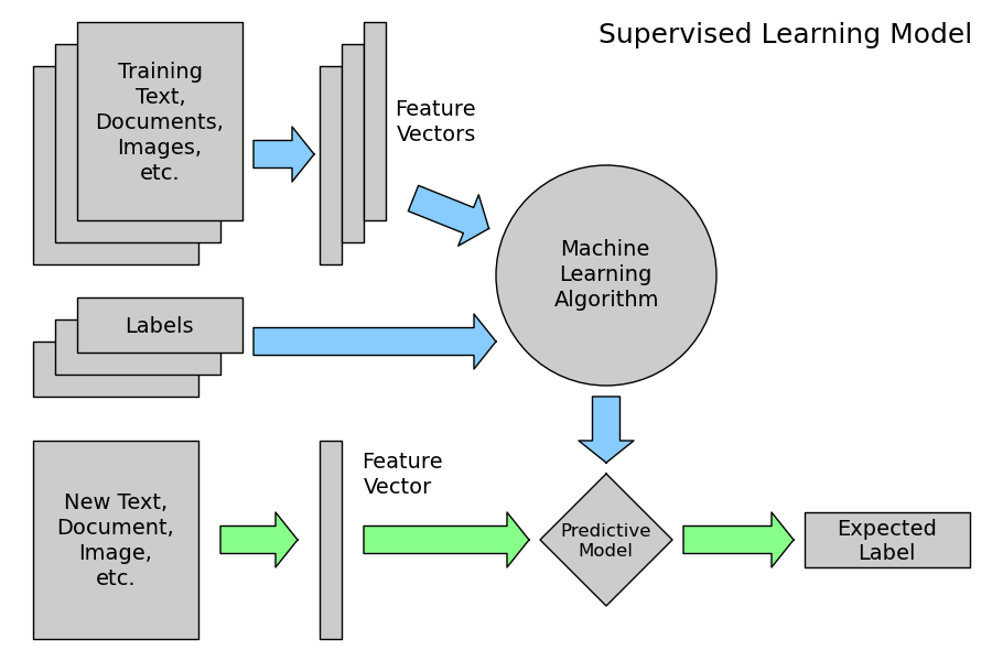
♣ 그리고 y label의 종류에 따라 classification & regression로 구분이 된다고 하였다.
- classification과 regression의 차이 -

♣ 여태까지 다룬 SLR, MLR, Ridge는 모두 y label이 연속적인 수치형인 'regression' model에 해당된다.
- classification도 매우 다양한 종류의 model 존재 -

♣ 이번 포스팅에서는 이와는 약간 다른 '지도학습 - classification'의 대표모델인 'logistic regression'에 대해서 알아보자
- 여기서 궁금증 -
Q) logistic REGRESSION인데 왜 classification algorithm인가요?
A) regression 모델을 기반으로 classification을 진행하는 모델이기에 이름에 'REGRESSION'이 들어가는 것일 뿐,
output type이나 모델 성능 평가 지표는 regression과 다르다는 점 꼭 기억하자!
1. classification → baseline model
✍️ 회귀문제에서는 보통 타겟 변수의 평균값이 기준모델로 사용되지만, 분류문제에서는 타겟 변수에서 가장 빈번하게 나타나는 범주가 기준모델로 사용된다
→ 따라서 우리가 구하고자 하는 타겟값이 모두 '빈번하게 나오는 값'일 경우의 모델 성능을 측정한다!
→ 그리고 이 성능보다 당연 높게 나오는 모델이 만들어져야 함
※ 주의 ※
<여기서 타겟 범주가 극단적으로 불균형 분포를 보이면, baseline model만으로 성능 측정 시 높은 정확도 값이 나온다. 따라서 불균형한 데이터를 가지고 모델 만들 때 주의!>
2. logistic regression
⭐️ 분류 알고리즘 중 대표적인 'logistic 회귀 모델'은 두 클래스 - binary class classify를 하는데 쓰이는 모델이다.
(세 개 이상의 class를 분류하는 분류 모델은 따로 존재! 추후 포스팅)
⭐️ 특히 스팸인지 아닌지 / 당뇨인지 아닌지 - 즉! A인지 B인지 두 개 class로 나누고 그 중 한 개를 결정하는 문제에 쓰임.
⭐️ binary classification problem에서 LR이 (이젠 편의상 Logistic Regression을 LR로 부르겠음) baseline model 자체로 쓰이는 경우도 있음
(↓↓↓ 아래 참고한 출처 일부 내용 발췌 ↓↓↓)
'Classification techniques are an essential part of machine learning and data mining applications. Approximately 70% of problems in Data Science are classification problems(많이 쓰이는 분류 문제). There are lots of classification problems that are available, but the logistics regression is common and is a useful regression method for solving the binary classification problem. Another category of classification is Multinomial classification, which handles the issues where multiple classes are present in the target variable. For example, IRIS dataset a very famous example of multi-class classification. Other examples are classifying article/blog/document category. Logistic Regression can be used for various classification problems such as spam detection. Diabetes prediction, if a given customer will purchase a particular product or will they churn another competitor, whether the user will click on a given advertisement link or not, and many more examples are in the bucket. Logistic Regression is one of the most simple and commonly used Machine Learning algorithms for two-class classification. It is easy to implement and can be used as the baseline for any binary classification problem. Its basic fundamental concepts are also constructive in deep learning. Logistic regression describes and estimates the relationship between one dependent binary variable and independent variables.'
⭐️ 위에서 말해주듯이 LR은 분류상 두 개로 나뉘는 binary variable (target) & 이 target을 위해 결정되는 여러 독립적인 변수들로 나뉨
(여기서 independent variable은 연속적이거나, discretized된 두 종류 모두 가능함)
⭐️ 아래 예시를 보면 independent variable이 'weight' 단 한 개일 때 obese한 지, not obese한 지 결정하는 classification 예이다.
-예시-

→ 위 그림에서 알 수 있듯이 빨간점 관측치가 여러 개 있는데 S자형의 로지스틱 회귀함수를 적용해서 단 두가지 범주! 비만인지 비만이 아닌 지를 결정한다. 👏🏻 (이런 함수를 생각해낸다니. 볼 때마다 경이롭다.)
<LR 식>
→ 이제 LR이 어떻게 기존 SLR에서 LR로 저렇게 S자로 변하는 지(또 그 반대는 어떻게 변환되는 지) 수학 식을 통해 자세히 확인해보자!
≪SLR → LR≫
SLR → S(x) sigmoid function에 대입 → 완성된 LR식!
◈ sigmoid ◈
→ 시그모이드 함수는 0에서 1사이의 함수로, S자 형태의 curve를 나타내는 함수이다. 주로 확률로 변환할 때 (확률이 0에서 1사이므로) 많이 거쳐가는 함수이며! 이를 LR에서 적용한다면, 관측치가 특정 class에 속할 확률값으로 시그모이드 형태 - 즉 S자형으로 나타낸다.
≪LR → SLR≫
반대로 LR을 SLR 직선형태로 바꾸는 걸 'logit transformation (로짓변환)' 이라 한다!
◈ Logit transformation ◈
→ 실패확률에 대한 성공확률의 비인 Odds(오즈)에 ln을 취하면 SLR 형태의 직선 방정식으로 바뀐다.
→ Odds = p/(1-p) (p는 성공확률)
→ 즉 성공할 확률이 1이면 Odds는 무한대, 성공할 확률이 0이면 Odds는 0
🙆♂️ odds 확률로 계산하려면 특성 X 단위로 1 증가시, odds확률이 exp(계수)배 증가한다고 말할 수 있다
🙆♂️ 여기서 예를 들어 odds가 3이면 성공할 확률이 실패할 확률보다 3배 더 높다고 해석하면 된다
→ 성공할 확률 = 정해진 기준값을 넘어 1이라는 부류에 속할 확률 (실제 모델에서 1과 0을 정확히 정해줘야 함)
(즉 이 '성공할 확률' p라는 건 LR값 자체를 말함! p = LR)
- odds비는 범위가 무한대이고 LR은 0에서 1사이! (직선과 곡선인게 차이점) -

- 위 두 변환을 아래 식으로 정리하면 다음과 같다! -
- (좌) SLR -> LR / (우) LR -> SLR -

⭐️ 정리하자면 기존 SLR을 시그모이드 함수에 집어넣어서 S자형으로 만든 새로운 LR모델을 만들어 낸다. 우리는 기존확률(default 0.5)보다 더 높은 값으로 확률이 측정되면 1, 아니면 0인 binary classification을 수행한다! 결과 0과 1로 나온 두 가지 부류를 새로운 예측결과값으로 집어넣는다 (총정리)
⭐️ 만약 그 반대로 logit transformation을 수행하면 단적인 SLR이 산출되어 회귀계수의 의미를 쉽게 해석할 수 있다
(그래서 본래 목적은 분류이지만 선형회귀 모델을 변형한 모델이므로 logistic REGRESSION이라 부르는 것이다)
⭐️ 이런 classification model을 결정하기 위해 MLE(Maximum Likelihood Estimation) 기법을 사용한다. SLR에서는 Least-Sqaure Method(OLS), 즉 거리의 최소화 기법으로 모델을 결정함. 즉, 모델 만드는 방법이 다름
⭐️ 추가로 linear model과 다른 점은, 더 복잡한 모델과 비교가 불가능하다는 점
- OLS는 저번에 배움 -

⭐️ MLE 기법 (너무 어렵기에👼 - MLE 기법에 대한 자세한 내용은 별도 포스팅 참조 - 곧 정복함.😉)
- 22.06. 26 정복했뜨아..! -
Maximum Likelihood Estimation(MLE)
🌟 로지스틱 회귀 포스팅에서 MLE기법을 통해 model을 결정한다고 하였다. 로지스틱 회귀의 식을 더 deep하게 수학적으로 들어가, 어떤 모델을 고를 지 수식으로 연산하는 과정에서 MLE가 핵심으로
sh-avid-learner.tistory.com
→ 확실히 여기서 알고 넘어갈 것은, MLE 기법에 의해 주어진 data에 대해 가장 잘 설명하는 S자 곡선을 찾게 됨!
'Binary Logistic Regression: The target variable has only two possible outcomes such as Spam or Not Spam, Cancer or No Cancer. & Multinomial Logistic Regression: The target variable has three or more nominal categories such as predicting the type of Wine. & Ordinal Logistic Regression: the target variable has three or more ordinal categories such as restaurant or product rating from 1 to 5.'
→ 우리가 배운 LR은 두 클래스만으로 나누는, 0과 1로 나누는 모델에 대해서 배웠는데, 세 가지 카테고리 이상의 nominal & ordinal target으로 나누는 LR 모델까지 존재한다는 점
(nominal, ordinal data - EDA posting에서 배웠슴)

+ requirements / advantages & disadvantages>
😻 requirements>
→ binary logistic 회귀 모델은 dependent variable의 개수가 2개이다.
→ dependent variable과 연관 있는 variable만 포함되어야 한다.
→ independent variable끼리는 서로 연관성이 없어야 한다. (다중공선성 배제)
→ 로그우도는 주어진 independent variable에 맞는 비율로 구성되어 있어야 한다.
→ 로지스틱 회귀에서 필요한 건 큰 sample size
😻 advantages>
→ 과적합이 빈번히 일어나지 않는 모델 (일어난다면, 위에서 제시한 대로 L1과 L2 규제 진행하면 됨)
→ 선형 구분 가능한(linearly separable) 특성으로 구성된 dataset이라면 로지스틱 회귀가 매우 효율적이다
→ neural network와 매우 비슷한 점을 갖고 있다. 여러 개의 조그마한 로지스틱 회귀를 모은 집합을 neural network라 할 수 있기 때문!
→ Artificial Neural Network와 같은 정교하고 복잡한 모델보다 training time이 적게 걸리는, 단순하지만 효율적인 모델
→ neural network의 뼈대를 이루고 있는 model이 로지스틱이라 할 수 있음!
→ softmax 함수를 이용한 멀티클래스 분류기로 확장 가능한 multinomial 로지스틱 회귀 모델이 있다.
😻 disadvantages>
→ 과적합이 일어나지 않게, independent variable 개수보다 적은 수의 observation이 있어서는 안된다
→ 로지스틱 회귀는 linear boundary를 그어 두 class로 분류하는 분류기이므로, 복잡하거나 non-linear 속성의 data로는 적용 불가능
→ 로지스틱 회귀는 discrete한 두 class로만 예측 가능
→ 큰 training sample이 필요한데 단 한 개도 빠짐없이 모든 training sample이 어떤 class에 각각 원래 속하는 지의 정보를 모두 알고 있어야 한다.
→ 이상치에 민감
→ 실제 세계(real-world problem)에서는 linearly separable 선형 가능한 data가 많지 않다. 더 복잡한 차원의 data가 대부분이므로, 해당 data를 feature의 개수를 높여(차원을 높인다는 뜻) linearly separable하게 만들어야 한다.
3. classification → Evaluation Metrics
⭐️ R2 결정계수 활용 불가 - OLS method로 산출하여 나오는 이 방식은 classification에서는 적용 불가능!
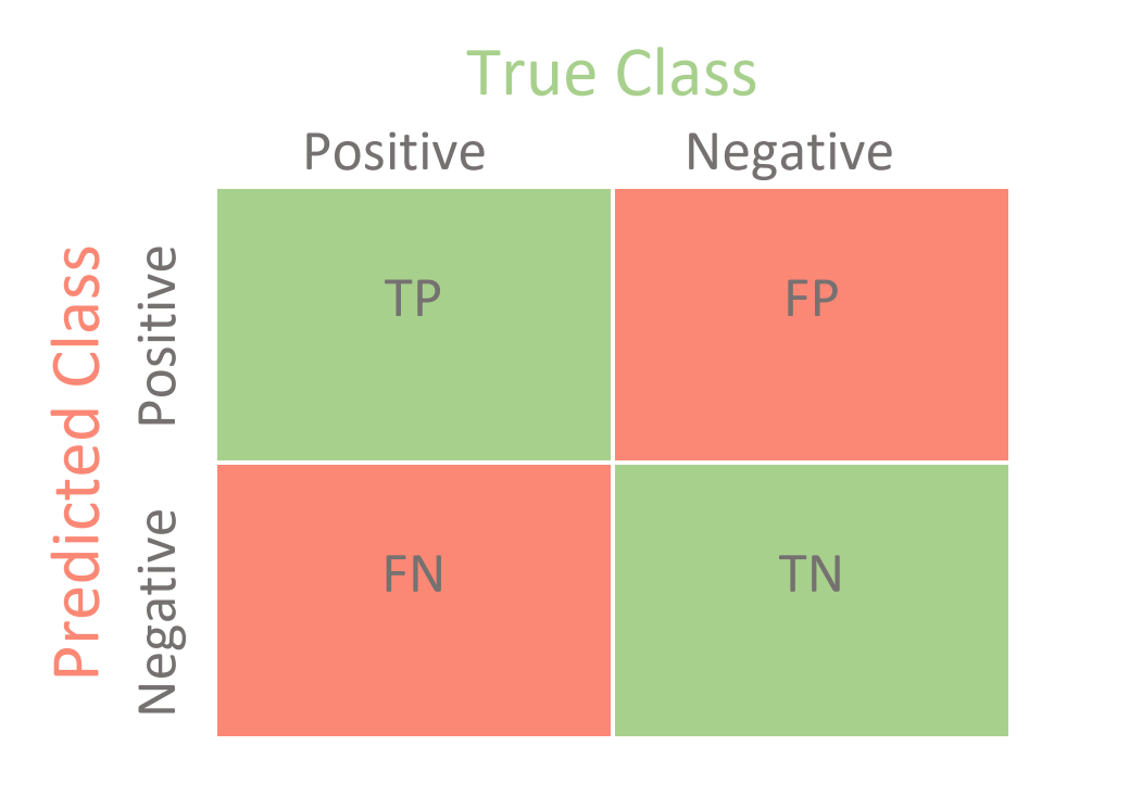
⭐️ 답은 '혼동행렬(confusion matrix)'
→ precision, recall, f-score, 그리고 accuracy라는 이 4가지의 새로운 평가 지표를 사용하여야 함
→ 아래 주어진 혼동행렬로 (0과 1을 예측한 것 vs. 실제 0과 1) 이렇게 네 개의 확률을 사용해 다양한 지표를 만들 수 있음
⭐️ metrics 수치로 어떤 특성이 target을 나누는 데 적절한 지 feature를 고를 수 있게 됨
- confusion matrix -
- 자세한 건 confusion matrix posting 참조 (추후 포스팅)-
4. logistic(lasso) + ridge
→ continuous, discrete variable일 경우 penalty를 가해 덜 과적합된 model로 만들어주는 ridge, lasso
→ 이 ridge, lasso 규제가 logistic model에도 적용이 가능하다.
* ridge> minimize할 비용함수
$\sum_{i}^{n} (y_i - \hat{y_i})^2$ + $\lambda$$ \sum_{j}^{p} \beta_j^2$
- 여기서 $\hat{y_i}$는 sigmoid 함수로 나타낸 P(X) (range 0~1) 값이며, 우리는 로지스틱을 만드는데 사용된 $\beta_j$인 여러 회귀계수 값을 줄임으로써(ridge 적용 결과 penalty 값 $\lambda$값이 커지므로) 덜 과적합된 로지스틱 모델을 구축한다.
* lasso> minimize할 비용함수
$\sum_{i}^{n} (y_i - \hat{y_i})^2$ + $\lambda$$ \sum_{j}^{p} |\beta_j|$
- 위 ridge와 똑같은 방식으로 덜 과적합된 로지스틱 모델을 구축할 수 있다.
- 간단한 개념 설명 끝! 🧙-
* 썸네일 icon) https://bigml.com/releases/summer-2016
* 그림 - 혼동행렬 출처) https://towardsdatascience.com/confusion-matrix-for-your-multi-class-machine-learning-model-ff9aa3bf7826
* 출처1) 🐣 갓 STATQUEST https://www.youtube.com/watch?v=yIYKR4sgzI8&feature=youtu.be
* 출처2) https://builtin.com/data-science/supervised-machine-learning-classification
* 출처3) https://scikit-learn.org/stable/modules/linear_model.html#logistic-regression
* 출처4) logistic regression 자세한 설명 https://www.analyticsvidhya.com/blog/2021/10/building-an-end-to-end-logistic-regression-model/
* 출처5) 데이터캠프 ☀️ https://www.datacamp.com/community/tutorials/understanding-logistic-regression-python
* 출처6) 시그모이드 설명 https://en.wikipedia.org/wiki/Sigmoid_function
* 출처7) ridge/lasso + logistic https://towardsdatascience.com/the-basics-logistic-regression-and-regularization-828b0d2d206c
* 출처8) classification model 종류 https://ogrisel.github.io/scikit-learn.org/sklearn-tutorial/tutorial/text_analytics/general_concepts.html#machine-learning-101-general-concepts
'Machine Learning > Models (with codes)' 카테고리의 다른 글
| Logistic Regression Model (w/code) (0) | 2022.04.25 |
|---|---|
| Polynomial Regression Model (0) | 2022.04.24 |
| (L2 Regularization) → Ridge Regression (w/scikit-learn) (0) | 2022.04.20 |
| (L2 Regularization) → Ridge Regression (concepts) (1) | 2022.04.19 |
| Multiple Linear Regression Model (concepts+w/code) (0) | 2022.04.17 |

댓글