🤹🏻♀️ 강력한 시각화 library seaborn의 세 개의 그래프 displot, pariplot, regplot에 대해서 알아보는 시간을 가져보려 한다.
🍡 seaborn.displot() docu
https://seaborn.pydata.org/generated/seaborn.displot.html
🍡 seaborn.pairplot() docu
https://seaborn.pydata.org/generated/seaborn.pairplot.html
🍡 seaborn.regplot() docu
https://seaborn.pydata.org/generated/seaborn.regplot.html
1> seaborn.displot
seaborn.displot(data=None, *, x=None, y=None, hue=None, row=None, col=None, weights=None, kind='hist', rug=False, rug_kws=None, log_scale=None, legend=True, palette=None, hue_order=None, hue_norm=None, color=None, col_wrap=None, row_order=None, col_order=None, height=5, aspect=1, facet_kws=None, **kwargs)
'This function provides access to several approaches for visualizing the univariate or bivariate distribution of data, including subsets of data defined by semantic mapping and faceting across multiple subplots.'
→ 한 개의 변수 또는 두 개의 변수 간의 데이터 분포를 시각화하는 displot() 함수이다.
Data Analysis with Python (2/2) (from Coursera)
4) Model Development * A Model = a mathematical equation used to predict a value given one or more other values - Relating one or more independent variables to dependant variables (ex) 'high..
sh-avid-learner.tistory.com
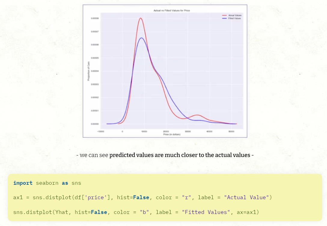
→ 위 coursera posting에서 두 변수의 분포를 표현하는 데 seaborn의 distplot을 사용하였는데, seaborn 버전이 업그레이드되면서 displot()으로 형태가 바뀌었다. 업그레이드되면서 더 다양한 형태의 분포를 시각화할 수 있게 됨!
- univariate -
→ 인자 kind에 세 개의 값을 넣을 수 있다
① 'hist(defalut)' - 히스토그램 생성
② 'kde(kernel density estimates)' - 히스토그램을 겉 테두리 선으로 그은 그래프라 생각하면 편하다.
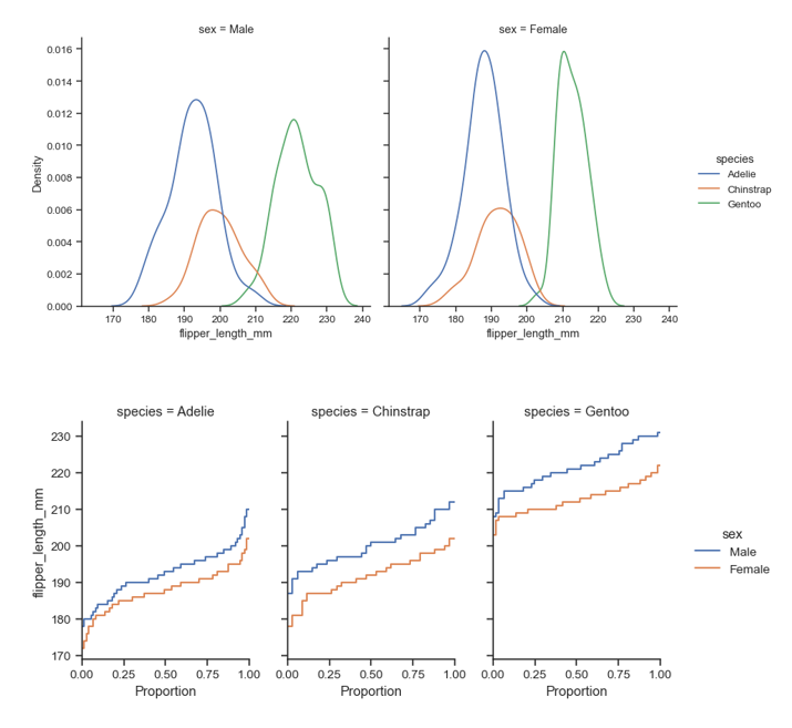
③ 'ecdf(empirical cumulative distribution functions)' - 누적 히스토그램의 누적값을 나타낸 그래프이다. (univariate만 표현 가능)
→ 위 1~3 그래프 예시를 보면 아래와 같음 (왼쪽부터 histogram, kde, ecdf)

→ 히스토그램에 kde 라인을 추가해서 겹친 형태로 시각화도 가능! (kde = True로 인자를 넣으면 됨)

- bivariate -
① default로 heatmap과 같은 형태가 출력된다 (두 변수 특정 구간에 해당되는 count가 높으면 더 진하게 칠해지는 형태로 시각화됨!)
② kind='kde'값을 넣으면 등고선의 형태로 빈도가 높은 쪽에 선이 많이 밀집되어 있는 형태로 출력됨
(추가로 rug값에 True를 넣으면 기존 등고선 그래프에서 밀집된 data를 각 축 별로 선을 통해 보여줌)

★ hue값을 통해 다양한 그룹의 data를 한 번에 한 개의 그래프로 분포 비교를 할 수 있다는 점! (※매우 중요 인자) ★
→ multiple = 'stack' 값을 넣어 하단 우측과 같이 겹친 히스토그램 형태로도 표현 가능 (딱히 사용하지는 않음!)

★ 한 번에 여러 개의 그래프, 즉 다양한 facet 형태를 출력해주어 시각화도 가능하다
※ 다중 그래프로 나눌 기준을 col 인자로 설정해 나눌 수 있음
2> seaborn.pairplot
seaborn.pairplot(data, *, hue=None, hue_order=None, palette=None, vars=None, x_vars=None, y_vars=None, kind='scatter', diag_kind='auto', markers=None, height=2.5, aspect=1, corner=False, dropna=False, plot_kws=None, diag_kws=None, grid_kws=None, size=None)
'Plot pairwise relationships in a dataset. By default, this function will create a grid of Axes such that each numeric variable in data will by shared across the y-axes across a single row and the x-axes across a single column. The diagonal plots are treated differently: a univariate distribution plot is drawn to show the marginal distribution of the data in each column. It is also possible to show a subset of variables or plot different variables on the rows and columns.'
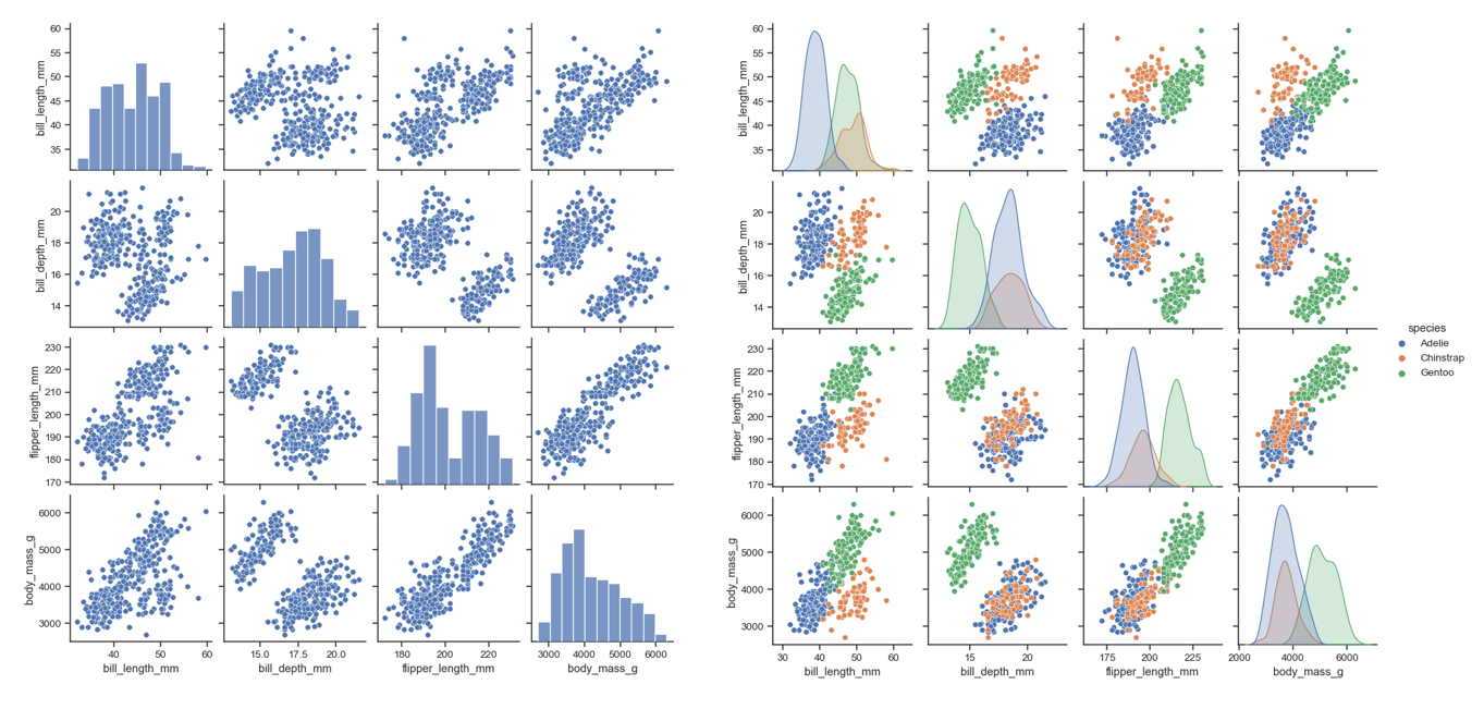
→ 위에서 배운 displot의 경우 단순히 분포 자체를 알 수 있는 시각화였지만, pairplot의 경우 두 변수끼리의 관계도 알 수 있다. 추가로, 왼쪽 대각선에 놓인 그래프들은 각 변수별 분포를 나타낸 것으로, displot보다 훨씬 더 많은 기능을 제공하는 시각화 plot이라고 할 수 있음!
★ 두 변수 간의 관계를 나타내는 그래프는 default로 scatterplot 시각화가 제공되며,
대각선 형태의 plot은 default histogram / hue값으로 그룹화하면 kde 그래프가 출력된다
(이 때, diag_kind값에 다른 그래프 타입을 hist값으로 넣어서 히스토그램으로도 출력 가능하다)
★ kind값에 kde, hist를 넣어 scatterplot이 아닌 다른 형태로 두 변수 간의 관계를 시각화할 수도 있다

★ 그 외로, x_vars와 y_vars에 일부 변수만 지정해 전체가 아닌 pairplot의 일부만 시각화도 가능하며,
markers값을 세부적으로 설정해 scatterplot의 점 형태를 달리 바꿀 수도 있음!
+ height로 각 세부 그래프들 높이도 설정 가능
+ corner = True값으로 왼쪽 대각선 기준 아래 그래프 (대각선 플롯 포함)만 시각화 설정 가능
그 외로 dict 형태로 인자를 집어넣어 customize 가능!
추가적인 다양한 형태는 이후 프로젝트에서 여러 시각화를 진행하면서 소개해 볼 예정이다 🏄♂️
3> seaborn.regplot
seaborn.regplot(*, x=None, y=None, data=None, x_estimator=None, x_bins=None, x_ci='ci', scatter=True, fit_reg=True, ci=95, n_boot=1000, units=None, seed=None, order=1, logistic=False, lowess=False, robust=False, logx=False, x_partial=None, y_partial=None, truncate=True, dropna=True, x_jitter=None, y_jitter=None, label=None, color=None, marker='o', scatter_kws=None, line_kws=None, ax=None)
'Plot data and a linear regression model fit.'
→ 예전에 linear regression 모델에 대해서 배운 적이 있다.
Simple Linear Regression (concepts)
** 우리는 저번시간에 Supervised Learning - Regression - Linear Regression까지 concepts에 대해 배웠다 (↓↓↓↓↓↓ 하단 포스팅 참조 ↓↓↓↓↓↓) ML Supervised Learning → Regression → Linear Regr..
sh-avid-learner.tistory.com
→ 주어진 data가 있으면 data의 추세를 반영해 한 개의 선으로 자동으로 시각화 해주는 plot (coursera 포스팅에서 아래와 같이 배움)

→ 일반적으로는 아래 좌측과 같이 그래프가 표현되고, confidence interval 수치를 더 줄여서 선이 포함되는 범위를 더 줄여 나타낼 수 있다 (우측)
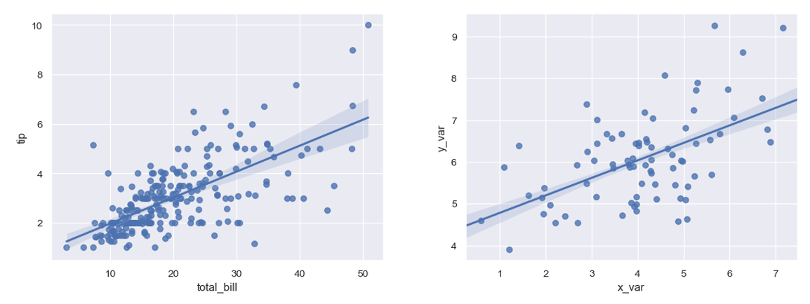
→ logistic 인자를 설정함으로써 로지스틱 회귀 모델로 시각화가 가능하기도 함!
🤾 총 세 가지의 seaborn plot에 대해 알아보았는데, 후에 직접 EDA 과정 또는 분석과정에서 여러 시각화를 사용할 때 많이 활용이 될 듯 하다!
- 개념 정리 끝! 🏆-
'Visualizations > Various Graphs' 카테고리의 다른 글
| Visualization - Graphs summarized (0) | 2022.05.02 |
|---|---|
| violin plot (+seaborn) (0) | 2022.03.27 |
| box plot (+seaborn) (0) | 2022.03.25 |
| folium 시각화 (0) | 2022.03.24 |

댓글